Don’t trust univariate feature selection

This has come up a few times in recent courses so I’m putting an explanation here with real code and data so that I have something to point people at. Given the complexities of feature selection, this may turn into a series!

Here’s a toy regression dataset. Imagine we have two features called x0 and x1 and an output that we’re trying to predict called y. Plotting the features shows that they are both noisily correlated with y:

You can download the dataset used below as toy_data.csv if you want to rerun the code yourself.

import pandas as pd
from sklearn.model_selection import train_test_split
from sklearn.feature_selection import f_regression, SelectKBest
from sklearn.linear_model import LinearRegression
from sklearn.metrics import mean_squared_error, r2_score

data = pd.read_csv("../datasets/toy_data.csv")

import seaborn as sns

sns.pairplot(data, x_vars=['x0', 'x1'], y_vars=['y'], kind='reg')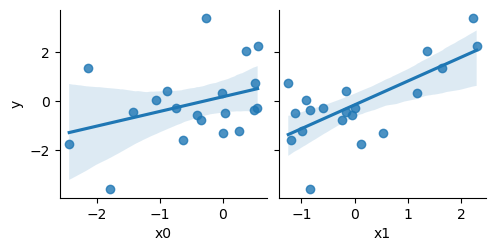

Now we will do the standard train/test split and divide into featues and outputs, leaving us with four variables:

train, test = train_test_split(
   data, test_size=0.25, random_state=42
)

len(X_train), len(X_test)

(15, 5)

We want to pick a single feature for fitting a linear regression, so we will calculate the F-score for each variable using the training set:

F, p = f_regression(train[['x0', 'x1']], train['y'])

print("F-scores:", F)
print("p-values:", p)

F-scores: [5.60840928 3.37168689]
p-values: [0.03404968 0.08929401]

The conclusion is straightforward; the first feature, x0, has the highest F-score and p-value. In a real sklearn workflow we might delegate this work to SelectKBest, which gives the same answer:

sel = SelectKBest(f_regression, k=1)
sel.fit(train[['x0', 'x1']], train['y'])
sel.get_feature_names_out()

array(['x0'], dtype=object)

However, when we try actually building a model with each of the two features individually, we get a much worse score with x0:

(
    LinearRegression()
    .fit(train[['x0']], train['y'])
    .score(test[['x0']], test['y'])
)

-2.121886807431179

than with x1:

(
    LinearRegression()
    .fit(train[['x1']], train['y'])
    .score(test[['x1']], test['y'])
)

0.1520767602584302

Why is this the opposite way round to what we expect based purely on the F-scores? Because we have been unlucky with the train/test split. Plotting just the test dataset shows that the correlation is much better for x1, the same as in the whole dataset:

sns.pairplot(test, x_vars=['x0', 'x1'], y_vars=['y'], kind='reg')

but in the training dataset, which we used for determining the F-scores, by chance the x0 correlation is better:

sns.pairplot(train, x_vars=['x0', 'x1'], y_vars=['y'], kind='reg')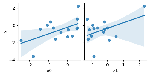

If we rerun the train/test split without the fixed random seed, and do the F-scores again:

train, test = train_test_split(
   data, test_size=0.25
)

F, p = f_regression(train[['x0', 'x1']], train['y'])

print("F-scores:", F)
print("p-values:", p)

F-scores: [ 5.05314215 20.18322846]
p-values: [0.04257063 0.00060546]

we get the correct conclusion; that x1 is the best feature.

In the real world, we might avoid this problem by doing cross-validation, to see which features are consistently selected, or by using F-scores as a preliminary filter and keeping a generous number of features to go into our real model.